


Every business needs customers, and successful businesses know they need a deep understanding of their customers to continue to grow. With a better knowledge of their buyers’ wants and needs, a business can create products or services that better meet (and exceed) their customers’ expectations, which means winning more deals and staying ahead of the competition. The more a business knows about their customers, the better they can operate their business.
There are countless important questions a business leader might ask about their customers to gain the insights they need. Often these questions are posed to the most logical source – analysts who have access to a variety of databases and information and are known for providing valuable easy-to-read visuals that leaders can take action on. Behind each of these questions is an analyst wrangling and interrogating data to find the answers. Today we explore a simple solution to summarizing a series of questions using the Dataiku Window Recipe.
A window recipe evaluates groups of records and produces summary values for each individual record in the dataset. For example, “How much more (or less) did a customer spend on their previous order?” With this ability to generate additional information while retaining the original dataset schema (i.e., more columns for every row), window functions are especially useful for machine learning tasks like time-series analysis and supervised prediction on transactional datasets (shopping, banking, etc.).
While some analytical questions can be answered through a combination of other functions (e.g. group-by’s and joins), we’ll see that the window function offers an efficient and elegant solution for a wide range of uses.
An Overview of Window Functions
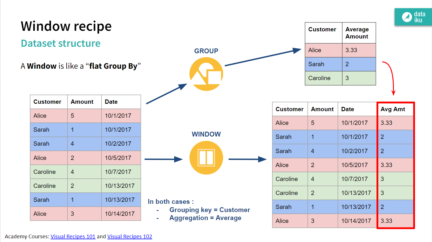
The Dataiku window recipe is based on the window function found in common SQL systems. A window function adds columns to the dataset and retains all existing information. This is different from a group-by function, where only summary information is returned, and the original structure of the dataset is lost. See the figure below from the Dataiku Academy that helps explain the difference between the concepts.
A window function has three components:
- Partition: the “grouping” key consisting of one or more columns
- Order: the column that sorts records within each partition
- (Window) Frame: limits the range of records included in the function evaluation
Depending on the task and intended summary information, one or more of these components may be required. For example, total sales by customer only requires a partition (by customer) and a summation of all sales records. If instead, you want to see cumulative sales over time, you need to include an order (e.g., date of sale). Further, if you wanted to see a rolling three-month sales total, you would need to add a window frame (again based on date of sale) that would include only the last three months of time up until the current record (date) being evaluated.
Based on the configuration of these window components (referred to as the window definition), many different analyses are possible resulting in a variety of summary information. There are three general types of analyses that window functions facilitate:
- Rankings - numbering of records
- Aggregations - grouping calculations
- Lags (Leads) - evaluating with prior/future records
People are usually most familiar with the “group-by” style of aggregations (min, max, average, sum, count, etc.), and these work as expected for window functions. Rankings are probably the most straightforward summary, as these simply assign a number (“rank”) to each record within each partition based on the order and an optional frame. However, there are several variations to how these ranks can be calculated, such as how to handle ties or duplicate records, which we’ll see later.
Perhaps the most useful feature, and uniquely specific to window functions, lagging (or leading) evaluations are used to compare the current record to previous (or future) records, such as the difference between values. These functions can also bring the value of these other records to the current record. For example, you could use a lag function on customer order dates to calculate the number of days since their previous order, as well as including the date of that previous order.
Next, we’ll walk through an example of each one of these types of window functions. Generally, these are all commonly used together, and over a variety of window definitions on the same dataset. With this ability to generate additional information while retaining the original dataset schema (i.e., more columns for every row), window functions are especially useful for machine learning tasks like time-series analysis and supervised prediction on transactional datasets (shopping, banking, etc.).
Choosing a Dataset for Our Window Recipe
In this tutorial, we will use a classic example database known as Northwind Traders. This synthetic dataset simulates the many operations of a small business that imports and exports specialty foods from around the world. Importantly, the database contains stereotypical examples of common business entities, and this allows us to illustrate common analytics use cases. Here we will focus on only a few aspects of the database, namely: customers, products, and orders. In essence, our simplified operating narrative is: customers make orders that contain some quantity of item(s) from the product list.
This dataset is small by today’s standards, but it serves well for our demonstration purposes. It contains 830 orders (2,155 line items) over 89 customers and 77 products. Within our Dataiku project, only minor preparation is used to combine the database tables (imported as separate CSV files) into analytics-ready datasets for our window recipes. Two datasets will be used in this tutorial: 1) “order-level” summary with one record per order (Orders_DetailRollup), and 2) “line-item” data with many records per order, where each line (record) is a specific product that is part of the sale (Orders_LineItems). See our annotated Dataiku project flow below. 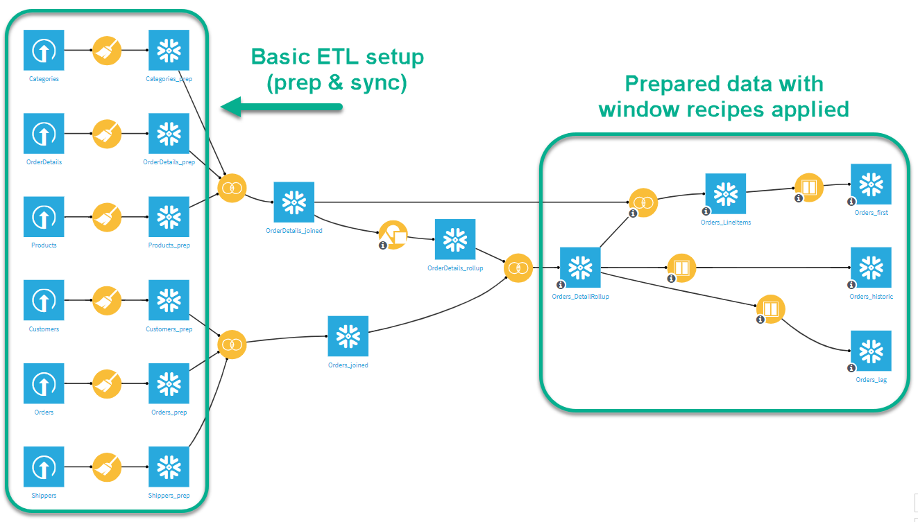 Note: The lore of Northwind Traders goes back decades to the original release of Microsoft Access, where it was included as an example database. Since then, it has remained a fixture in the database community, popping up as an example database/dataset in a variety of formats. We based our dataset on the extended version, which we extracted from SQL scripts to CSV files and uploaded directly into our Dataiku project. For more information, check out https://en.wikiversity.org/wiki/Database_Examples/Northwind.
Examples: Windows Recipe Applied to Business Sales Data
We present three questions a hypothetical business might ask about their sales data. For each question, we show how to set up a window recipe to find the answer and explore the resulting dataset. We also include a chart to visualize the results. It’s important to remember how valuable visualization can be for communicating data, and Dataiku makes this simple from directly within the dataset explorer interface.
Question 1: What is the first product our customers usually order?
Let’s break down the question to better see how the window function fits. We can start by identifying the first order for each customer. We partition the data by customer, order by order date, and apply a ranking to number the orders. Then we filter to keep only rank #1 records (first orders), counting all the products in just those orders.
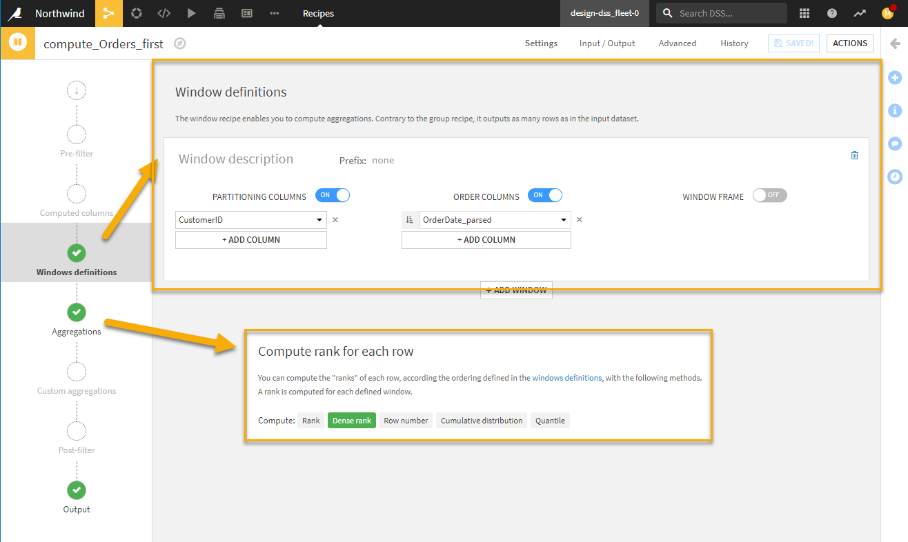
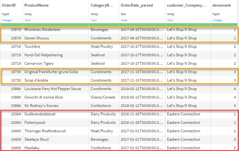
The figure below shows the visual recipe setup for the “Windows definitions” and “Aggregations” tabs. The other tabs are unmodified. Notice we chose Dense rank, which allows for ties and contains no sequential gaps. We’ll perform this window query on the Orders_LineItems dataset, which means we will have one or more records for each unique order (based on order date here). Therefore, we want all records (items) in the first order to be ranked 1, then all the records in the second order to be ranked 2, and so on. After running the recipe, we can see the new ranking working as expected in the resulting dataset explorer window.
While we could filter on the column denserank to be equal to 1 at any time, we saved it for the chart filter. Now you can analyze products from any ranked order (e.g., “what do they buy on their 2nd or 3rd purchase?”) by simply changing the filter here or using the column value elsewhere in the flow. Lastly, we provide a horizontal bar chart below showing the top products found in the most first orders. We also use the product category column to add color groupings to the products for additional information and potential insight. Here we see that Raciette Courdavault (Dairy Product) is the most frequently purchased product in a customer’s first order.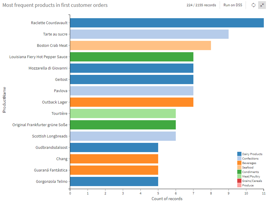
Question 2: How many orders have our customers had over time?
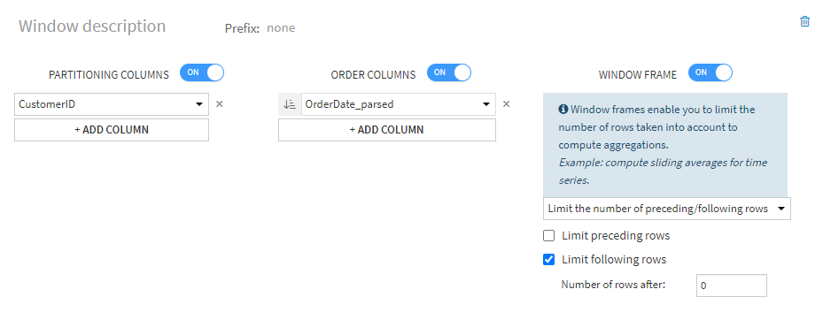
When we hear “over time,” it typically means historical and cumulative. We can set up a window frame to only evaluate previous records, which requires ordering the window by order date. Then we can count the number of orders for each customer over time and append this value to the dataset. Additional information for each order, like a customer’s historical number of orders, total items purchased, total dollars spent, etc., could be very useful in machine learning tasks too.
Similar to the last example, we partition on customer and order by order date, but this time we turn on the window frame. Then we select the checkbox limit following rows and enter 0 for “number of rows after”, which means that when given a specific record, we compute our aggregations on the current record and no records that follow it. Because limit preceding rows is not checked, that means that we will include all previous records too. This is where the partitioning and ordering columns play a crucial role in setting up the frame correctly. For example, if we reverse the ordering column, then the most current records would be at the top, and therefore, the historical records would actually be the “following rows.”
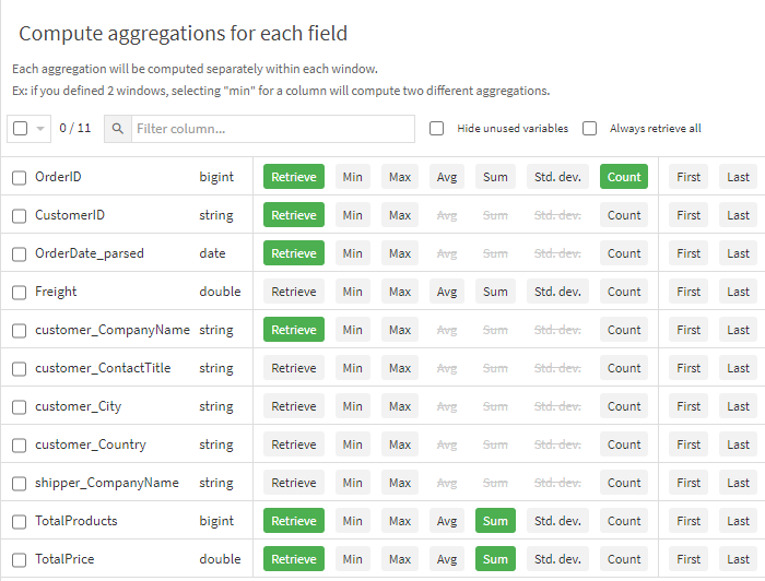
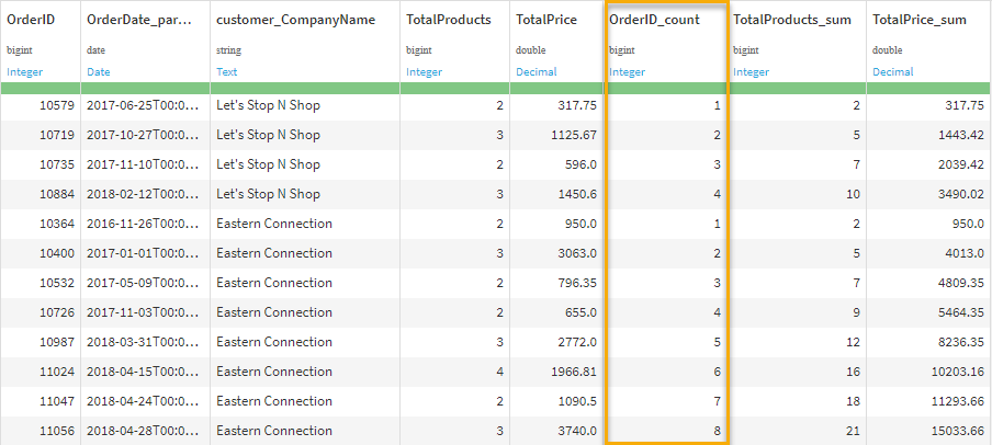
We selected three aggregation fields to include as new columns and optionally chose to discard some of the original columns (by unselecting the default Retrieve button). While we’ve been saying a window function retains the exact dataset schema, here we see it does not strictly have to, which is simply a matter of convenience for us. We can look at the resulting dataset and see all three of these new columns; notably our count of OrderID provides us the order number, and the sum of total products and total price provides the others, respectively.
Lastly, a line plot below presents the data for the top 15 customers, showing their total number of orders over time. We can see the top three (Save-a-lot Markets, Ernst Handel, QUICK-Stop) stand out from the rest, which could be an opportunity for further analysis.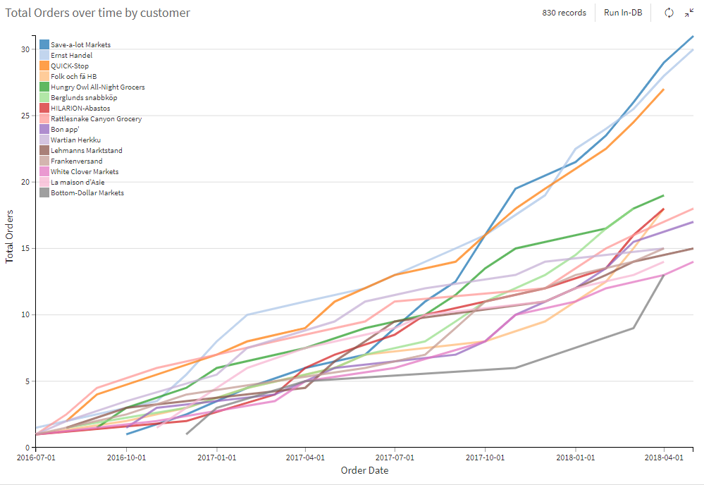
Question 3: How frequently do our customers make orders?
While this may sound similar to the prior question, a “frequency” here implies a comparison between events, which we can achieve with a lag window. Essentially, we can look at the time difference between consecutive orders (using the order date) for each customer. Because the lag values are associated with each record, we can then summarize them for each customer in our final answers and visualization.
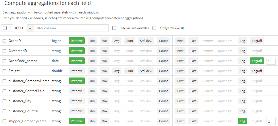
Here we set up the window the same as Question 1, partitioning on customer, ordering on order date, and disabling the window frame. For the aggregations, we utilize the LagDiff feature and give it a value of 1 (for comparing against the first row previously). We also include the Lag feature for shipper_CompanyName as an additional example of where lag values could be used for comparison. We can see the results of the lag columns in the output dataset below. Notice a lag means that the first record in each partition will not have a value. 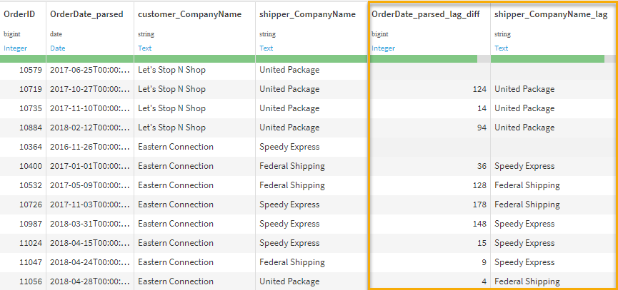
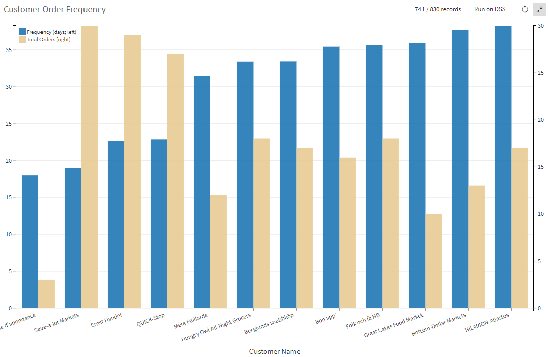
Lastly, we present this information as a bar chart where we include both the order frequency (in days) and the total orders for each customer, sorted by the most frequent. As expected, the top three order makers from question #2 are also at the front of this list, except for a customer with only a few orders that must have occurred very close together. This is a good example of a small sample size adding noise to a result; as is to be expected in real-world analysis.
Analytical Tasks Streamlined Through Windows Functions
Window functions can be a very useful tool for common analytical tasks. Using Dataiku’s visual window recipe, anyone can perform these operations without needing to write code. Most importantly, analysts can use this tool to help business stakeholders answer important business questions and more deeply understand their customers.
As you can see, no code software can open doors to a variety of efficiencies, automation, and insights for organizations and their data experts. Looking for more no-code tips? Find our best practices and options for transforming raw data into insights without coding knowledge in our recent blog.
| FEATURED AUTHOR: MIKE SCHUH, PHD
-1.png?width=290&name=Blank-Template-Facebook-Post%20(2)-1.png)